[Note this post is a bit outdated, and not maintained; the most up-to-date version of this information can be found in my pages on the OEIS wiki.]
I’ve recently become interested in a family of interrelated sequences that can be found in the Online Encyclopedia of Integer Sequences (OEIS). These sequences all have to do with one approach to measuring the “complexity” of an integer. This approach assumes that you have some basic “building blocks” for constructing integers: starting numbers you’re allowed to use, and operations that you may apply to them. The idea, then, is that the number of these building blocks that you need to arrive at a particular integer is one way of characterizing how “complex” that integer is.
This approach to constructing integers may seem familiar from the “Four fours” puzzle: Given four instances of the number 4 to start with, and a variety of operations that you might use, how many different whole numbers can you construct? For some examples, \[1 = \frac44 \quad 2 = \frac{4+4}4 \quad 3 = \frac{4+4+4}4 \quad 5 = 4+\frac44 \quad \ldots \quad 8 = 4 + 4 \quad \ldots \] Here it seems quite reasonable that in terms of “expressing with fours,” the number eight is “simpler” than the number three.
The lowest-numbered sequence (that I’ve found) in the OEIS that has to do with integer complexity is A000792. In the case of this sequence, the only number you’re allowed to start with is one, and the only operations you’re allowed to use are plus and times. The $n$th entry of sequence A000792 then tells you the largest number you can produce using at most $n$ ones.
Formally, let $A$ be an “alphabet” of numbers and operators; for simplicity we’ll assume all operators are unary or binary. One can then form finite sequences of elements from $A$; such a sequence is a well-formed RPN expression if no initial subsequence has as many binary operators as numbers. Each well-formed RPN expression unambiguously determines its value: imagine you have an initially-empty stack of numbers, and go through the sequence from left to right. Any time you encounter a number, put it on top of the stack; when you encounter a unary operator, modify the top number on the stack by applying that operator; and when you encounter any binary operator $\ast$, remove $a$ and $b$ (respectively) from the second-to-top and top positions from the stack, and then put $a\ast b$ on top of the stack (reducing the height of the stack by one). The value of the RPN expression is the top number on the stack when the entire expression has been scanned. The well-formed condition guarantees the stack never empties.
We can now define the $A$-operand complexity of a number $n$, which we’ll write as $c_A(n)$, as the minimum number of numbers in any well-formed RPN expression with value $n$, the $A$-operator complexity $d_A(n)$ as the minimum number of operators in any well-formed RPN expression with value $n$, and similarly the $A$-expression complexity $e_A(n)$ as the minimum length of a well-formed RPN expression with value $n$. There is no general relationship between $c_A$, $d_A$, and $e_A$, but if $A$ contains only binary operators, then $e_A(n)$ $= 2c_A(n)-1$ $= 2d_A(n)+1$. (Briefly, count the number of operators needed to reduce the operands to a single number; clearly the minimal expression in any case ends with a stack of just one number.)
Since it’s the most common notion of complexity used in the OEIS, we take “complexity” without an adjective to refer to $c_A$, the $A$-operand complexity.
I’ve also assembled a table that organizes sequences in the OEIS related to these notions of integer complexity, according to the alphabet $A$ and the particular measure or property of the complexity.
In both the Woven SSD and the Woven GSD, you calculate the inset (from the points where the rods meet near their ends) for putting marks on the rods by multiplying their lengths by 2/(3+√5). Where does that strange-looking number come from?
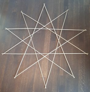
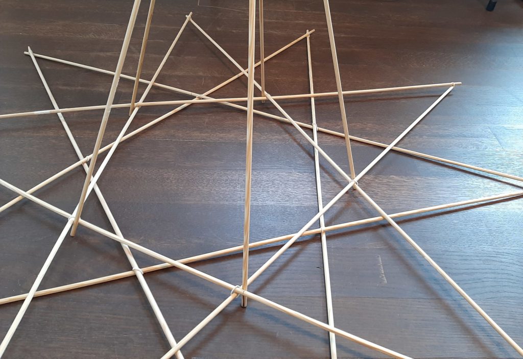
The key is that both figures consist of (regular) pentagrams, just interlocked in different ways. In other words, in both structures, looking only at any 5 rods in the same plane, we see:
What we’re interested in the fraction of the length of one rod (that is, the length between the points of the star where the rods cross; we’ll ignore the small overhangs beyond that from here on) represented by the distance from a point to the first internal intersection. In other words, we want the ratio of the red segment to the green segment in this diagram:
Now imagine that these segments are roads, and you start driving in a car from the red-blue point, and you follow all five of the roads until you end up back where you started, pointing in the same direction. You make five turns through the angle $\alpha$ indicated in the diagram below, but end up overall making two full turns all the way around (i.e., overall your car turns through an angle of $720^{\circ} = 4\pi = 2\tau.$) Therefore, $5\alpha = 2\tau,$ so the angle $\alpha = 2\tau/5,$ or 2/5 of a turn. We can then conclude that the point angle $\beta$ in the following diagram must be $\tau/2 – 2\tau/5 = \tau/10,$ or one-tenth of a turn (36 degrees).
The same argument applied to a regular pentagon shows that its interior angles are $3\tau/10$ (or 108 degrees). In other words, in the following diagram, the edges of the pentagram trisect the vertex angles of the circumscribed pentagon:
This angle relationship in turn means that the orange-pink-green triangle is similar to the brown-purple-green triangle. But it’s also clear that the long green is the sum of the brown and the purple. This similarity tells us that the sum of the purple and brown is to the orange as the purple is to the brown. But the orange is clearly the same as the purple, so the sum of the purple and brown is to the purple as the purple is to the brown. And this is exactly the definition that the purple cuts the long green in the golden ratio $\phi,$ i.e. that the purple is $1/\phi$ as long as the long green.
On the other hand, the brown-purple-green triangle is also similar to the acute pink-blue-red triangle. Applying the exact same argument as before shows that the red segment is $1/\phi$ as long as the purple segment.
Combining these two facts tells us that the red segment is $1/\phi^2$ as long as the long green segment. By solving the equation $(\phi+1)/\phi = \phi/1$, you can find the value $\phi=(1+\sqrt5)/2$. Using this value and some algebraic manipulations lets us calculate that the red segment is $2/(3+\sqrt5)$ as long as the green one, as used in the posts linked above.
This post was for announcing a week-long summer workshop on Illustrating Mathematics at the Park City Mathematics Institute, this past 2021 July 19-23. It was an exciting week with lots of interesting programming including several different hands-on, how-to tutorials, keynotes by Vernelle Noel, Ingrid Daubechies, and Daniel Piker, and mathematical “show-and-ask” sessions in which a wide array of mathematicians displayed some of the intriguing and beautiful images and objects they’ve created, as well as highlighting the questions these projects have raised. (I led one minicourse on using CAD/CAM software like LibreCAD or FreeCAD in creating physical mathematical models.)
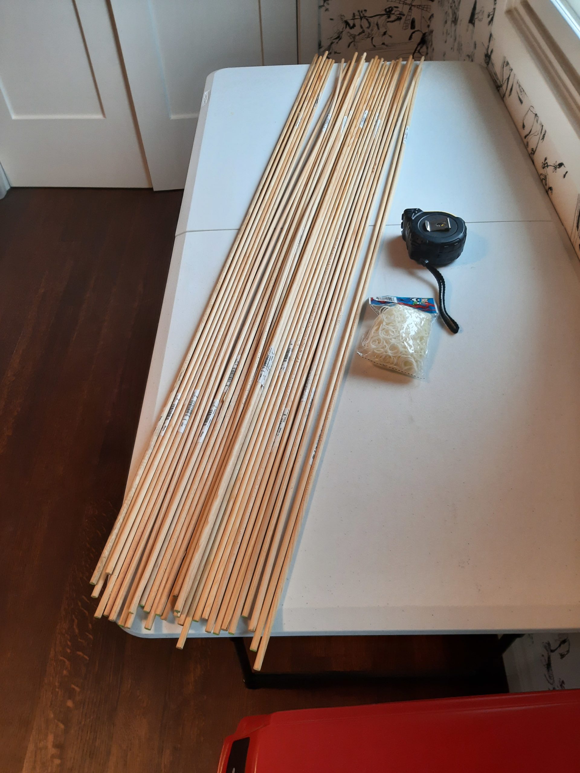
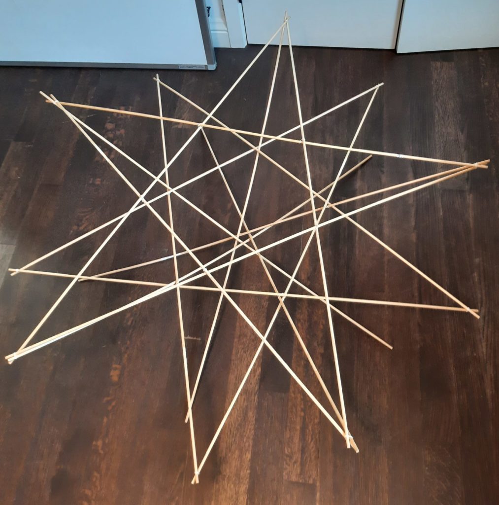
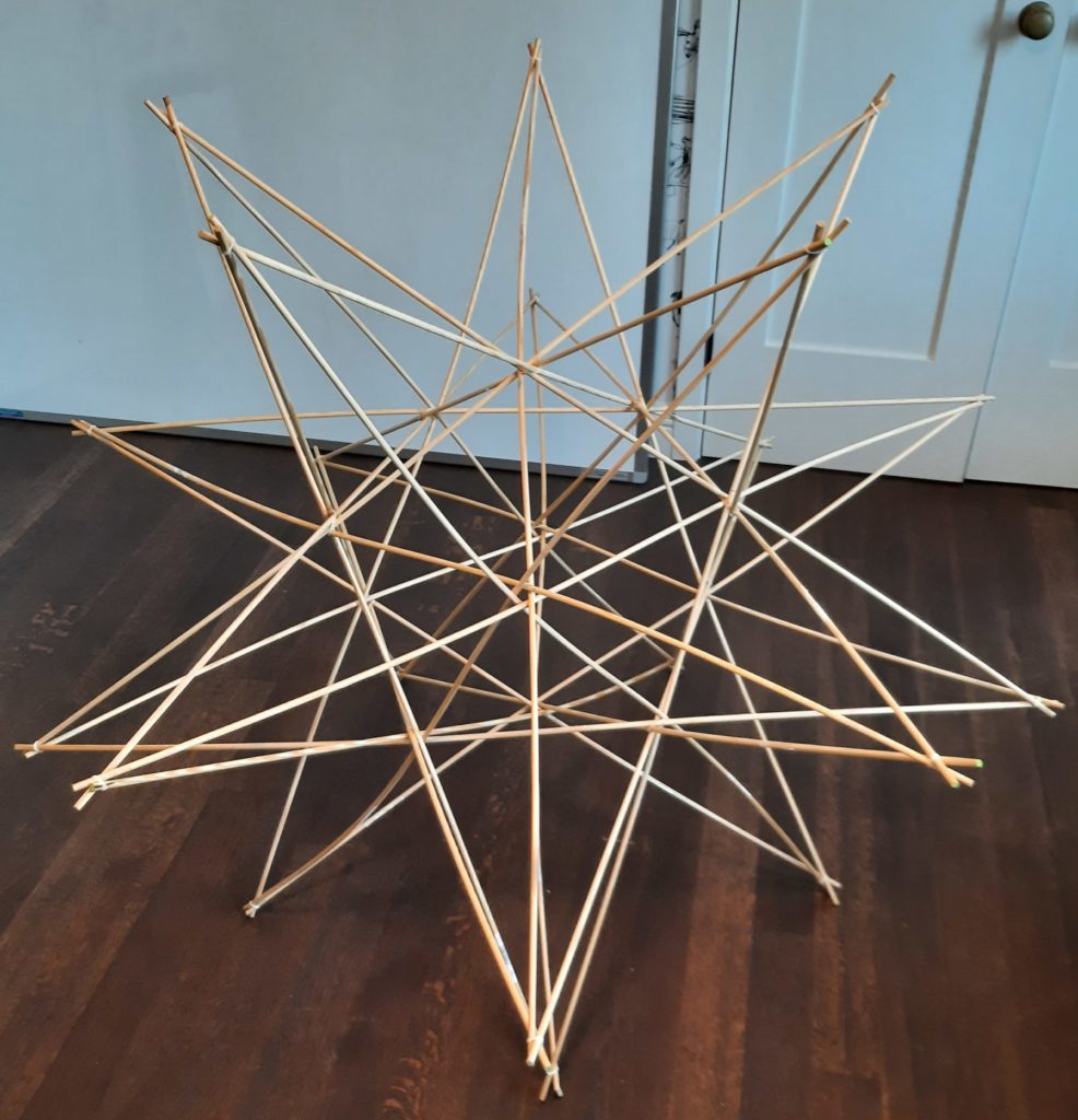
This is a sequel to a (pre-pandemic) post about weaving a stellated polyhedron. This time, I’d like to show how similar techniques can also be used to create a “great stellated dodecahedron” (“GSD” for short; illustration to the left). The materials are in fact the same as before, as summarized in the table above. This time, I am using 4-foot quarter-inch pine dowels for the rods, and white mini “rainbow loom” rubber bands.
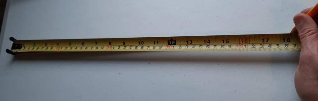
Begin by marking the same points on each rod as described in the previous post; in this case, with 48″ rods and allowing 1 inch of overlap at the ends, this is 1+(46 × 2/(3+√5)) or about 18 1/2″. (See this MathStream post for an explanation of where 2/(3+√5) comes from.)
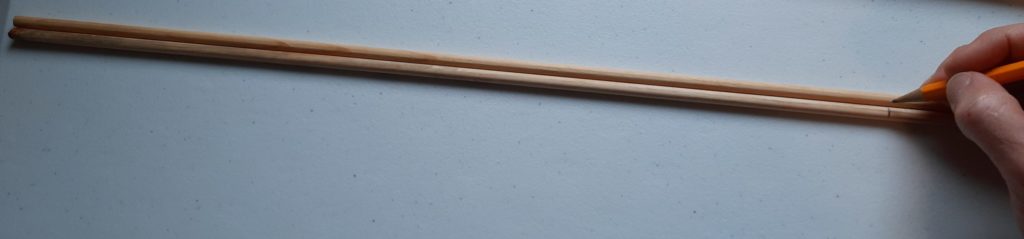
With rods this long, it’s easiest to transfer the marks from one rod to the next.
Once all of the rods are marked, make two five-pointed stars as described for the SSD, except both of these should have the reversed over-under pattern: As you follow a given stick around the inner pentagon clockwise, it must be on top at its first junction and on the bottom at its second junction. That means also that looking at any point with the center of the star away from you, the rod that comes into the point from the right should be on top. When both stars are done, put one on top of the other so that the points alternate:
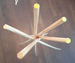
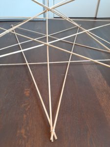
(Here the star with the point directed straight up in the picture is on top.) Now take five of the rods, stand them on end, and put a rubber band around them at the higher mark. Splay them out so that the top sections make a clockwise “whorl” when viewed from above:
Stand this “penta-pod” up amidst the two stars, with each leg just to the right of a corner of the inner pentagon of the top star:
Then slip the bottom of each leg into the rubber band at the junction it’s nearest, keeping it in the same relative position to the two horizontal rods crossing at that junction:
Now slide the top star up into the air, with each leg of the penta-pod sliding through the rubber band it was just inserted into. The legs will splay out as you do this. Keep sliding until the top star has reached the lower mark on each leg and these rods have spread out to reach the points of the lower star:
Finish this step off by inserting each leg into the rubber band at the point of the star where it’s ended up. You slide it in on the left, so that the three rods that meet at the point make a counterclockwise whorl. (As they will at every outer point of the GSD in the whole construction.) At right is a picture focused on one of the points, which will hopefully make the attachment clear.
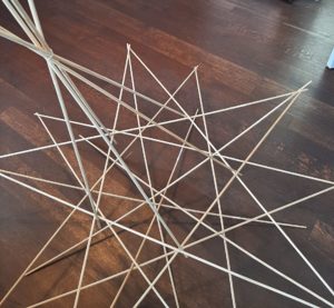
To prepare for the next step, make another “clockwise whorl” of five rods banded together at their top marks, just like the one you made before. When that’s ready, turn the construction over and rest it on what were the top ends of the five rods from the first whorl. The construction may sag a bit, but it should hold up and balance on the five ends of the rods. The two stars should still be quite close to horizontal, with the formerly lower one (that has three rods at each point) now above the other. Overall, the construction should look something like this:
Now insert each leg of the second whorl just to the right of one of the inner junctions of what’s now the top star, as shown at left. Below right is a view of all five ends inserted.
Slide all five of these legs through the rubber bands you just inserted them into, until they reach a point of the lower star. Once there, insert the leg into the rubber band at the point of the star in exactly the same way as you did with the first “pentapod” legs. See the detail picture below left:
At this point the structure should be symmetric from top to bottom. There are five unattached rod ends sticking upwards in a pentagon, and the structure is resting on five unattached rod ends at the bottom. The ends of these rods, together with the ten points of the first two stars, comprise the 20 outer vertices of the final GSD. The star points already have all of the rods attached that they will have at completion. There are ten unused rods remaining. Each one of these will extend in a straight line from one of the top five points, through two inner junctions (one from the top star and one from the lower star), and end at one of the lower five point. From each top point, there will be one rod extending down and to the right and one extending down and to the left; and arriving at each bottom point will be one rod from the right and one rod from the left. All that remains is to feed the rods through properly so that they are woven uniformly at each junction. They should create clockwise whorls at each inner junction (when viewed from outside the GSD), and as mentioned earlier, counterclockwise whorls of three rods at each outer point of the GSD.
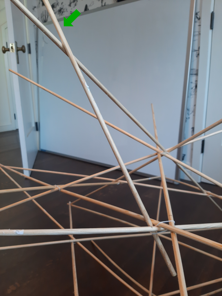
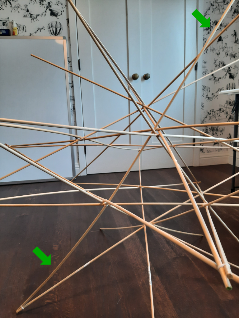
Here are some guidelines and pictures that should help to feed these rods through properly. We’ll begin with a rod (indicated by the green arrow in the following picture) that will extend down and to the right from one of the top points (at the extreme top left in the picture). It should feed through the inner junction of the top star that is immediately below and to the right of the top point; that’s the one with the white rubber band in the lower foreground of the picture. Specifically, it will feed through the leftmost sector of this junction:
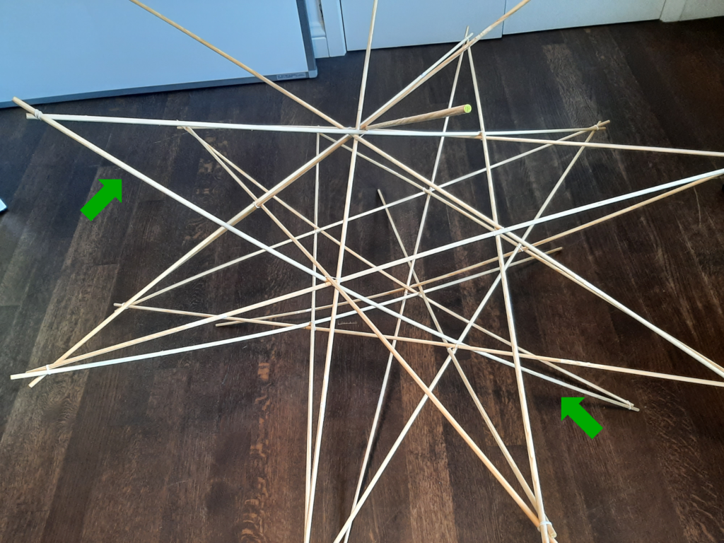
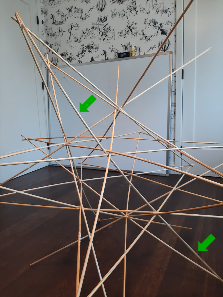
It then feeds through the inner junction of the lower star just below and to the right of that, but this time it feeds through the rightmost sector of that junction. The new rod then proceeds down to the end of the lower leg that’s just below and to the right of that. The next picture shows just the one new rod added, in its final position. The new rod is again indicated by green arrows; pay particular attention to how it passes through the two inner junctions: all the way on the left at top, and all the way on the right for the lower one.
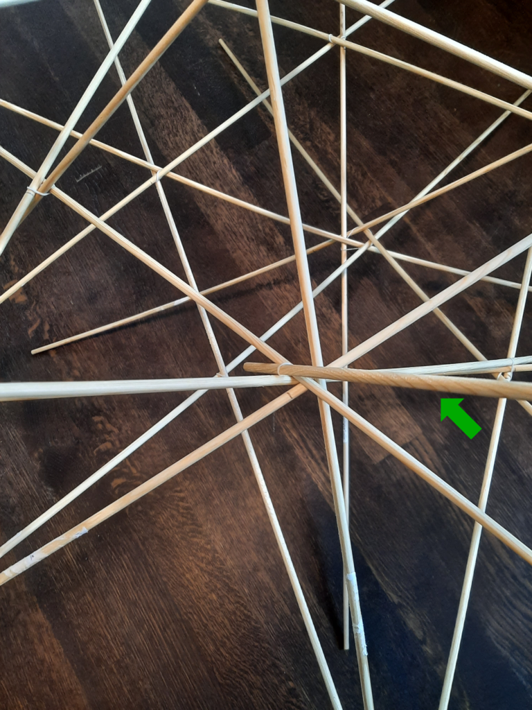
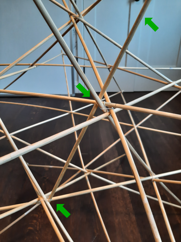
The next rod we’ll feed through will run from the upper point next counterclockwise (as viewed from the top) from the one we just attached to, and proceed to the left through the same inner junction that we just used. This will add the fifth and final rod to that particular inner junction of the upper star. As with the previous rod, we’ll insert it in the leftmost sector of that junction. Here’s the rod (we’ll continue indicating the newly-added rod with green arrows for the rest of the post) just after it’s been properly threaded through the rubber band at that inner junction of the top star:
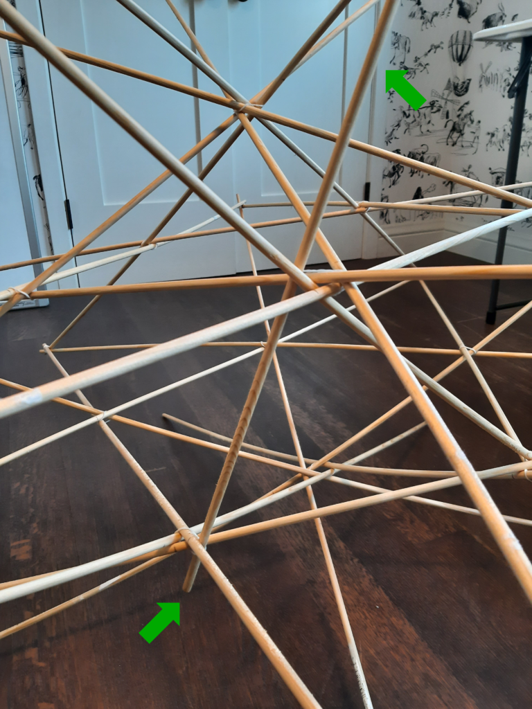
Keep feeding it through until it reaches the inner junction of the lower star just to the left; there, as before, feed it through the rightmost sector of the junction:
Once it’s through that rubber band, continue feeding it until it reaches the end of the bottom leg below and to the left of that junction:
Make sure you secure it at the top as well. Now you’re in the home stretch — just eight more rods to insert. It’s most straightforward to insert them in pairs, just like the previous two, rotating the structure one-fifth of a turn before each pair to orient the location for their insertion toward you. Here’s the structure after just one more rod has been inserted:
For every rod that you insert, it feeds through the leftmost sector of the junction where it passes through the top horizontal star, and the rightmost sector of the junction where it passes through the bottom horizontal star. You can see this again in the following picture of the fourth rod in the midst of being inserted: (125302 goes here)
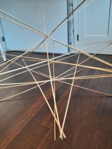
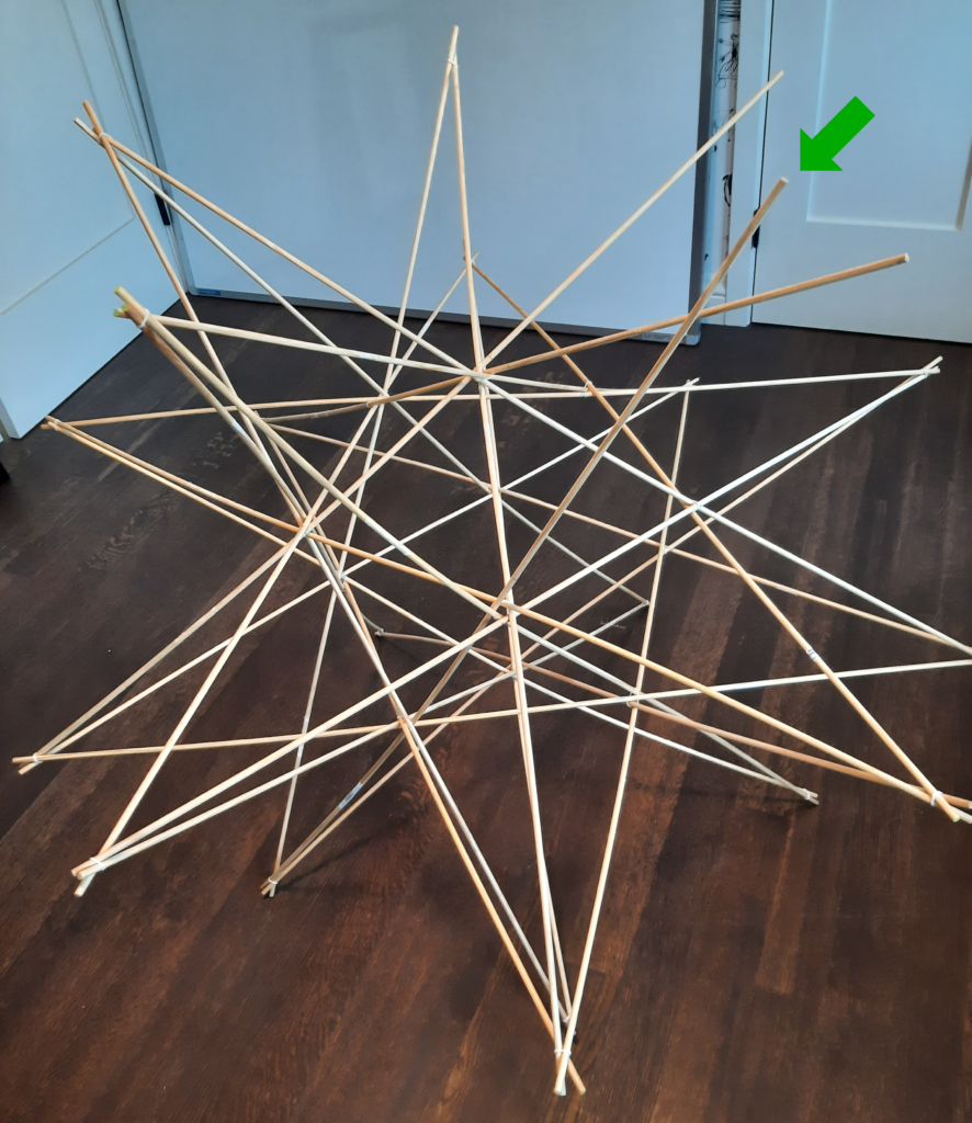
You should also see a regular icosahedron begin to emerge at the core of the GSD. Here’s a view just before the sixth rod is secured to its top point:
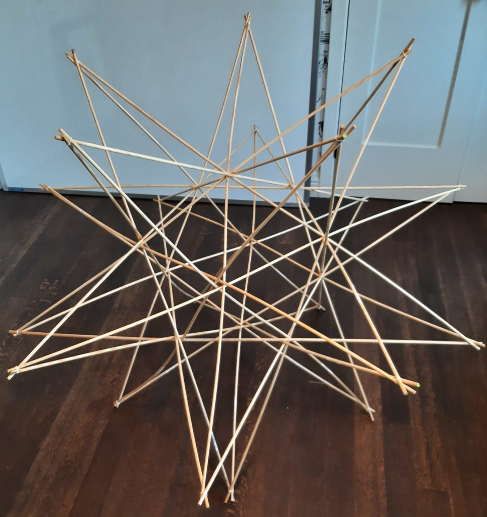
If you just keep going in this same fashion for all ten of the last group of rods, you’ll complete the star. Here’s a view just after the last rod is inserted:
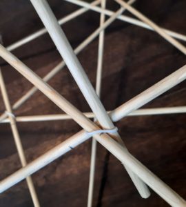
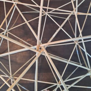
And now you’re pretty much done! There’s really only a couple more optional steps you might want to do to get your great stellated dodecahedron into optimal shape. As depicted at right, you can examine and gently adjust each of the inner junctions of five rods (that form the vertices of the inner icosahedron) to ensure that each one makes a tidy regular pentagon at the five-way crossover. In addition, if you’ve built your GSD from rods with even a moderate amount of surface friction (dowels, paper straws, even metal rods), you can now snip the rubber bands off of all of the interior, five-way junctions and the GSD will hold together just fine. (Theoretically, you can cut the outer rubber bands at the points where three dowels come together as well. If you want to try this, I recommend just trying a couple of widely-separated ones at first, and leaving off if the outer junctions don’t seem to be holding up well. I pretty much reserve this for stars built out of really highly frictional items or ones that can be twisted a bit at the outer points, like pipe cleaners.)
It’s a bit of an involved building process, but I think the elegance and symmetry of the final construction are well worth the effort. Here’s a picture of the final result with inner rubber bands removed:
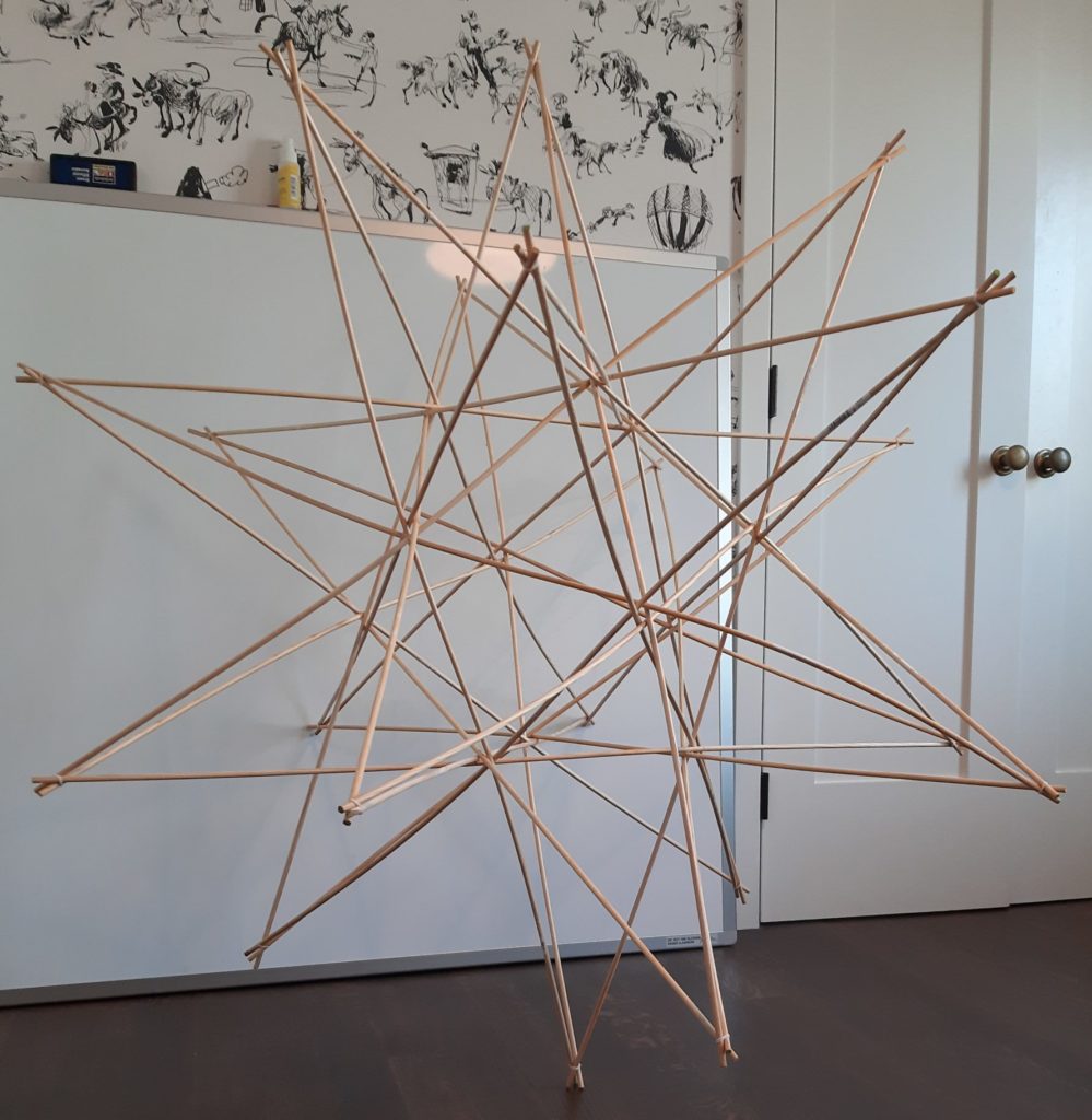
In addition, you’ll find that the finished GSD is surprisingly sturdy and robust. You can easily pick it up and handle it without fear of it falling apart. As an illustration, here’s a closing shot of the great stellated dodecahedron supported on just one point:
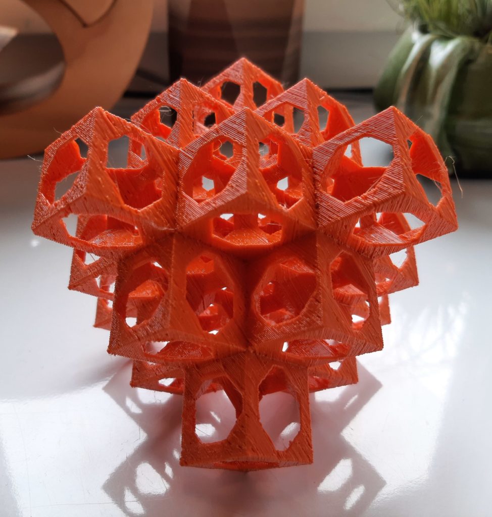
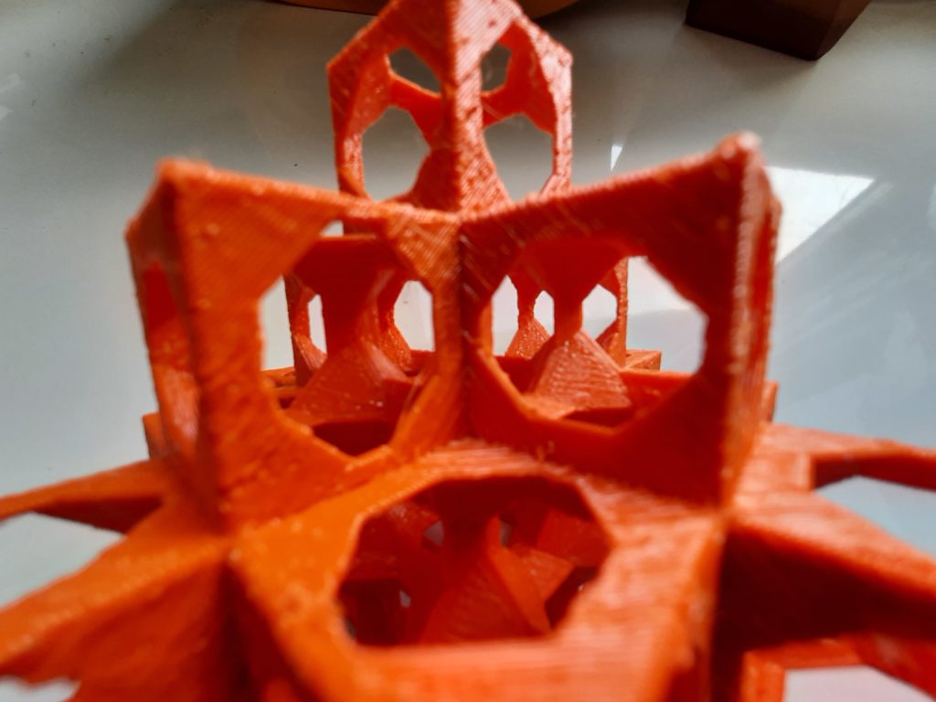
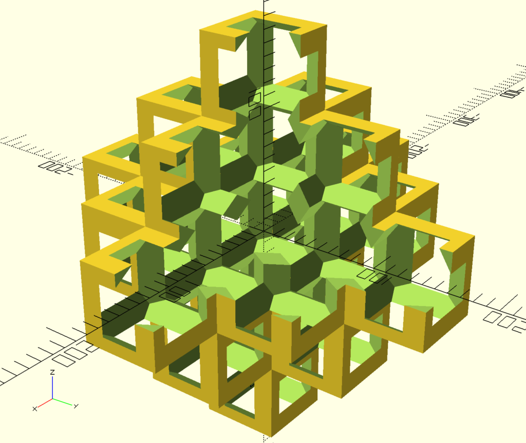
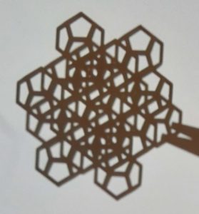
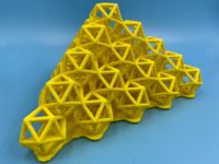
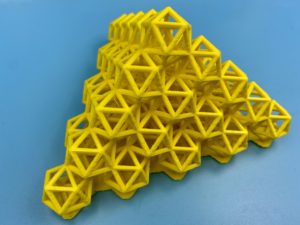
After seeing Laura Taalman’s inspiring 3d print, it occurred to me that one could also render the edge-to-edge cubical array of dodecahedra contemplated in this earlier post in an analogous way. Plus, I just received a new Prusa SL1 printer, and needed something to try it out on. So after just a bit moretinkering in OpenSCAD, and 400 minutes of print time using the resulting STL file, I ended up with this model:
If you recall, the negative space of the dodecahedron array was just a bit too monotonous to seem worth printing. However, I think that simplicity works very much to advantage in this wire-frame style of rendering. This model has enough complexity to afford visual richness, but is open and orderly enough not to be overwhelming.
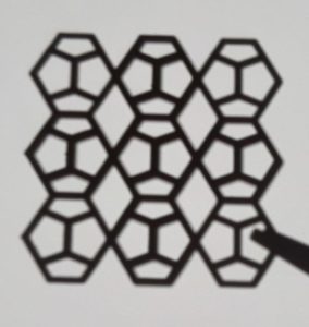
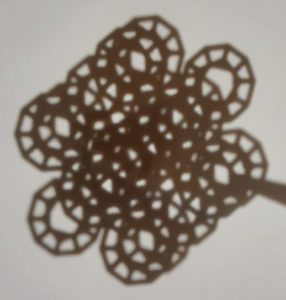
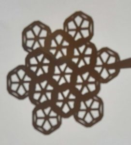
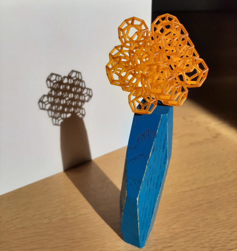
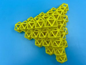
In addition, it produces an excellent variety of shadows (or parallel projections, in more math-y lingo):
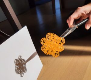
(The rhombuses in the top left photo correspond to the rhombic prism channels in the antidodec that we previously modeled.) Here’s another shot so you can see the setup for capturing the shadows. This is really best done in direct, bright sunlight — it’s tough to get such crisp, parallel rays of light otherwise.
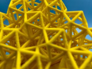
I can’t resist one more take on this lovely model and its shadows.
If you print one of these or a variation on it, I’d love to see/hear about it.
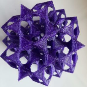
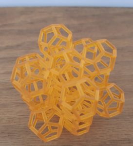
When I showed this recent post to my friend and colleague Laura Taalman, aka mathgrrl, she suggested that another approach to creating a model of the underlying structure would be to construct the icosahedra themselves (rather than the negative space), except use wireframes of the icosahedra rather than solid ones to avoid obscuring all of the internal structure. Her encouragement motivated me to create a new OpenSCAD file for this. Taking pity on the small size of the build plate of the 3D printer that I have access to, Laura even printed the resulting STL file for me. Her machine produced the following lovely results:
Whichever one you like better, this or the Anticos, I think it’s safe to say that the two models bring out different aspects of the same edge-to-edge arrangement of icosahedra. For example, this “wirecosahedra” structure shows better how the edges of neighboring icosahedra coincide. On the other hand, I think if we had only produced this model, it would be hard to discover the octahedra lurking in the corners between the icosahedra — they get a bit lost among all of the edges.
Thanks to Laura for providing another perspective on this arrangement of Platonic solids!
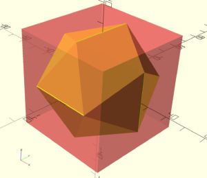
If you look again at the diagram of an icosahedron in a cube (at the right), you’ll see that because of its symmetry, all three of the icosahedron vertices nearest the top front cube vertex are the same distance from that cube vertex. That equidistance means that the body diagonal of the cube passes through the center of the icosahedron and is perpendicular to the nearest face of the icosahedron.
All of these properties hold at every vertex of the cube in relation to one of the eight faces of the icosahedron that do not have an edge lying in a face of the cube. Because the eight faces of the inscribed dual octahedron of the cube have these same properties, we’ve demonstrated that an icosahedron may also be inscribed in an octahedron like so:
It also means that if you extend the plane of one these particular eight faces of the icosahedron, it slices off an isosceles right triangular pyramid from the corner of the cube:
In a lattice of such cubes, eight of these pyramids fuse together at each vertex to create the octahedra seen inside the Anticos.
As mentioned and illustrated in the post on the Anticos, it’s possible to inscribe an icosahedron in a cube. (In this case, that technically means that given a cube, you can choose two points on each face of the cube such that the convex hull of the resulting set of twelve points is a regular icosahedron.)
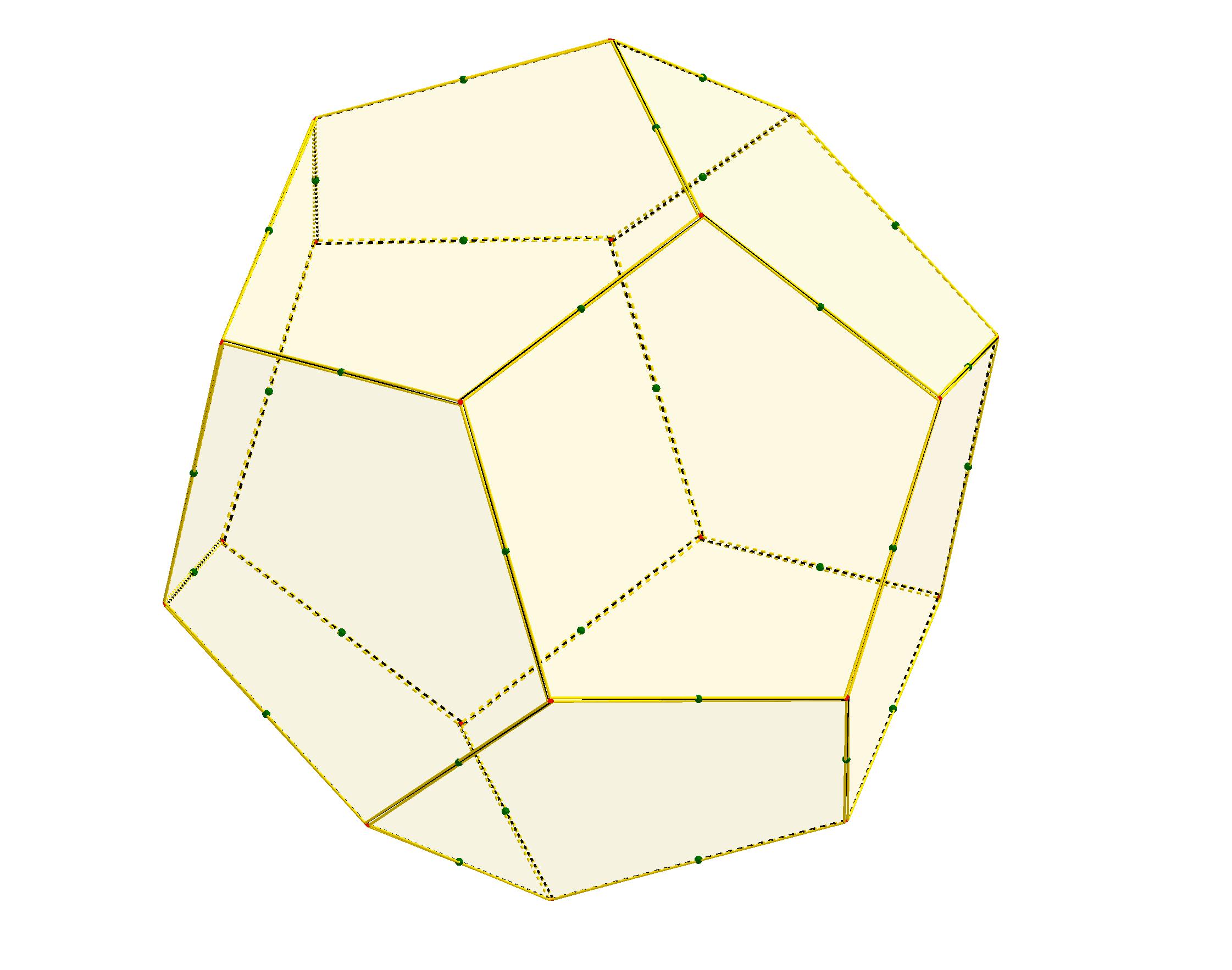
But why should this be so? To see this, it’s easiest to start with a regular dodecahedron, say with unit edge length. Notice the interesting pattern of the blue face diagonals in this diagram:
GIF
Notice that during this transformation, each of the edges remains in the plane perpendicular to that axis. Therefore, twelve of the vertices of an icosahedron lie on the surface of a cube, two on each face. Since an icosahedron only has twelve vertices, it is inscribed in a cube.
Judging from at least one of the previous projects, Studio Infinity is intrigued with connecting polyhedra edge-to-edge. (Of course, connecting them face-to-face is interesting, too, but that’s pretty familiar from Legos and such; and vertex-to-vertex is the same as connecting dual polyhedra face-to-face.)
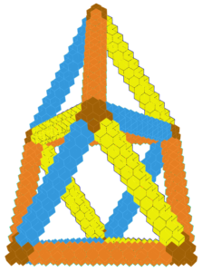
As you can see in the “blueprint” for the Boxtahedral Tower at right, connecting solids in this way often highlights symmetries that might otherwise be overlooked. In that case, edge-to-edge connections illuminated the threefold symmetries of cubes.
Even more surprising is that the most spherical of the Platonic solids, the icosahedron, can nestle into a cube with six of its edges just brushing the faces of the cube:
That means that if we connect icosahedra edge-to-edge, we should be able to make rectilinear structures, like with ordinary building blocks:
I wanted to find a way to show what was going on in this structure; but it seems as though the individual icosahedra get in the way of seeing the overall picture. You can’t see many of the actual edge connections at once.
Sometimes, however, what’s not there is even more illuminating than what is. Thus, the “Anticos” emerged: the negative space of the above configuration.
(More precisely, I enlarge each icosahedron by about 35% before carving it out of its respective cube. That step creates the “windows” in the sides of the cubes that lets you see the internal structure — without the enlargement, there would just be an infinitesimally narrow slit in each surface, so you would see nothing but a stack of cubes.)
Although usually S∞ focuses on structures that you can build by hand with ordinary materials, for something this intricate and detailed 3D printing seemed to be the only reasonable route to get a physical example in a reasonable amount of time. So here is the OpenSCAD source file and the resulting STL file. Since all of Studio Infinity’s content is Creative Commons-licensed, feel free to modify however you may like, and print if you have access to a 3D printer.
Now the icosahedra are revealed to embed in a lacy network of octahedra connected by rhombic prisms:
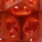
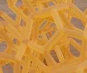
Although after the fact it may not be a mathematical surprise that octahedra show up between the icosahedra, it’s still visually striking, and I’d say that creating the physical model heightens our appreciation of how they all fit together. Moreover, physical models can reveal other surprising aspects of the underlying geometry. For example, this half-height prototype of the Anticos reveals a lovely network of hexagonal cross-sections of the packed icosahedra:
Hopefully, S∞ will have much more to say about connecting polyhedra both face-to-face and edge-to-edge in the weeks to come.
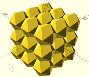
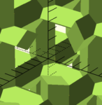
This MathStream post about why an icosahedron inscribes in a cube also shows that a dodecahedron fits into a cube in an analogous way. That raised the prospect that it might also be worth building an “Antidodec” analogous to the Anticos. So I quickly mocked one up in OpenSCAD (here’s the twofiles you need), producing the following image of what it would look like:
Surprise! it’s just a rectilinear network of (infinite golden) rhombic prisms. While it’s striking and lovely in its own way that this structure turns out to be so simple, it didn’t seem that the result would be visually interesting enough to be worth producing physically. So in the end, this post is really just a footnote to the prior project.
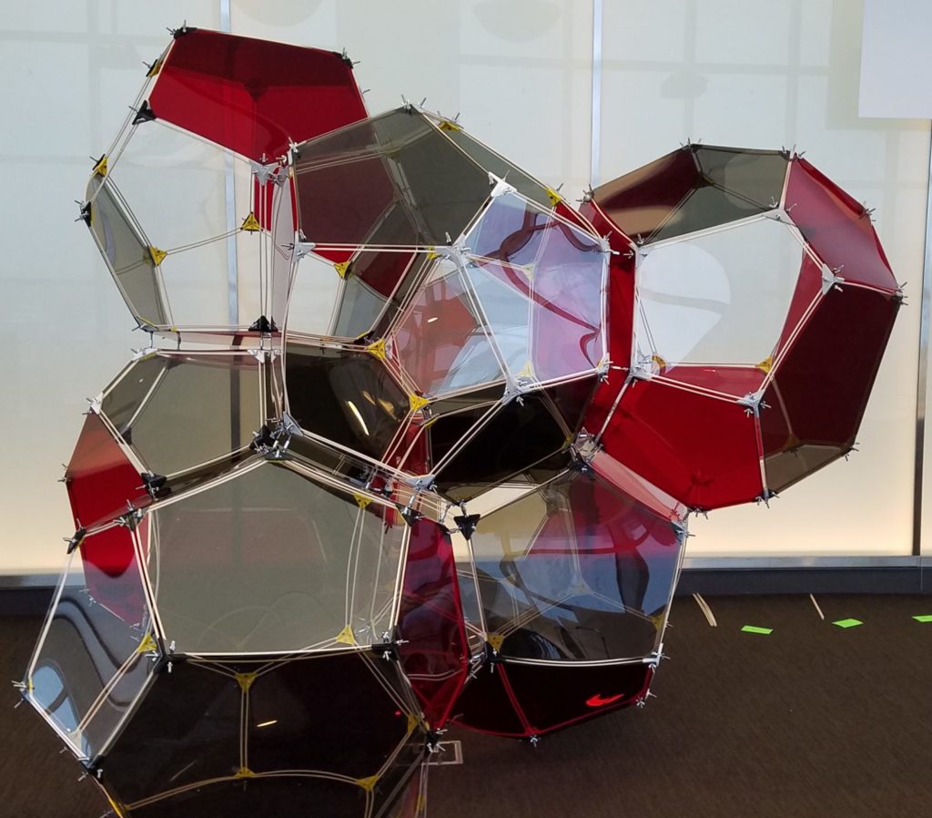
Here’s a large-scale model I designed of the Weaire-Phelan space packing, built by the participants of the Fall 2019 semester on Illustrating Mathematics at ICERM in Providence. The title above is a reference to the fact that it is still not established whether this is the most surface-area parsimonious way to divide space into cells of equal volume, like an ideal foam in which each bubble encloses the same volume.
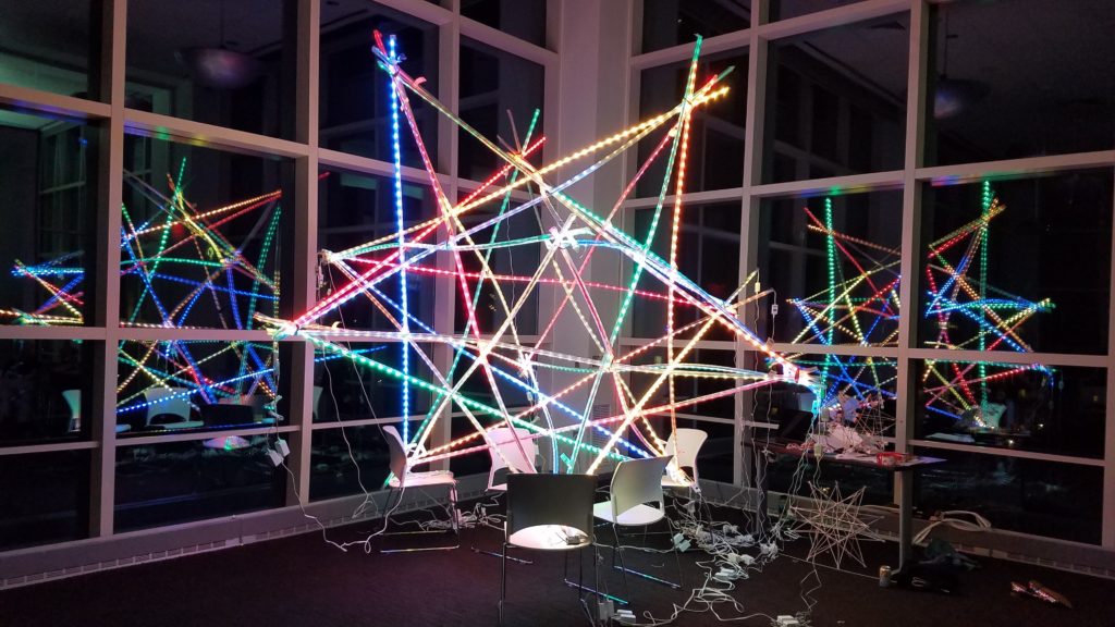
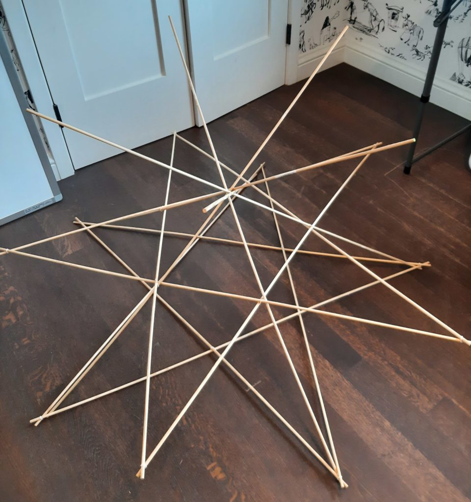
Here’s a picture of FireStar, a large-scale woven small stellated dodecahedron constructed by visitors to the open house of the Institute for Computational and Experimental Mathematics during Providence, RI’s WaterFire festival on 2019 Sep 28.


 are enough to guarantee that the blue figure is precisely a cube.</p>
<p>Moreover, it’s also clear from the diagram that the red edges are parallel to the faces of this blue cube. (By the symmetries highlighted in the last paragraph, both endpoints of a red edge are the same distance from the nearest face plane of the cube.) Therefore, if we expanded the cube slightly, each red edge would lie in a face of the cube. In other words, a regular dodecahedron has a property very similar to the one we are looking for concerning the icosahedron. (Which begs the question of what the Antidodec would look like — an <strong>S∞</strong> project for another day!)</p>
<p>We want to transfer this property to the icosahedron. Now, the dodecahedron is the dual of the icosahedron. And one, perhaps slightly less well-known, way of passing from a regular polyhedron to its dual is to rotate each edge a quarter turn around the axis connecting its midpoint to the center of the polyhedron:</p>
<div class=)